Archive for the ‘Climate’ Category

“But measuring rainfall is very tricky,” – Kerry Emanuel

August 19, 2013

It’s the tail wagging the dog, or the cart before the horse as the IPCC prepares to publish its report.

It’s the brave new world of Global warming – though global temperatures have been still or have declined slightly over the last 17 years. But it is 95% certain – says the IPCC –  that carbon dioxide is the cause and the world has warmed by 0.8 °C since the 1950’s. But that 95% is plucked from the air. But they are certain – from their models that the world will warm by upto 4°C in the next 100 years — and that carbon dioxide is the cause! We know the cause but we don’t know the effects!

The local effects are elusive.

“But measuring rainfall is very tricky,” said Kerry Emanuel

Reuters: 

Experts surer of manmade global warming but local predictions elusive

Climate scientists are surer than ever that human activity is causing global warming, according to leaked drafts of a major U.N. report, but they are finding it harder than expected to predict the impact in specific regions in coming decades. ….

…. Drafts seen by Reuters of the study by the U.N. panel of experts, due to be published next month, say it is at least 95 percent likely that human activities – chiefly the burning of fossil fuels – are the main cause of warming since the 1950s.

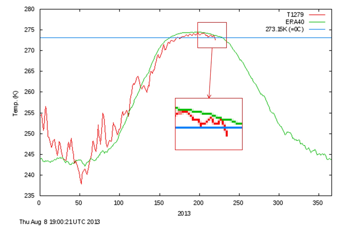
But they will merely ignore the real observation that global temperatures have not increased for at least 17 years.

“We have got quite a bit more certain that climate change … is largely manmade,” said Reto Knutti, a professor at the Swiss Federal Institute of Technology in Zurich. “We’re less certain than many would hope about the local impacts.”

And gauging how warming would affect nature, from crops to fish stocks, was also proving hard since it goes far beyond physics. “You can’t write an equation for a tree,” he said.

How exactly the certainty increased when temperatures did not go up while carbon dioxide concentration continued to increase is of no consequence – apparently. How certainty increases when the models are diverging more and more from reality is another mystery.

The IPCC report, the first of three to be released in 2013 and 2014, will face intense scrutiny, particularly after the panel admitted a mistake in the 2007 study which wrongly predicted that all Himalayan glaciers could melt by 2035. Experts say the error far overestimated the melt and might have been based on a misreading of 2350.

The new study will state with greater confidence than in 2007 that rising manmade greenhouse gas emissions have already meant more heatwaves. But it is likely to play down some tentative findings from 2007, such as that human activities have contributed to more droughts. ….

Drew Shindell, a NASA climate scientist, said the relative lack of progress in regional predictions was the main disappointment of climate science since 2007.

“I talk to people in regional power planning. They ask: ‘What’s the temperature going to be in this region in the next 20-30 years, because that’s where our power grid is?'” he said.

“We can’t really tell. It’s a shame,” said Shindell. Like the other scientists interviewed, he was speaking about climate science in general since the last IPCC report, not about the details of the latest drafts.

WARMING SLOWING

The panel will try to explain why global temperatures, while still increasing, have risen more slowly since about 1998 even though greenhouse gas concentrations have hit repeated record highs in that time, led by industrial emissions by China and other emerging nations.

An IPCC draft says there is “medium confidence” that the slowing of the rise is “due in roughly equal measure” to natural variations in the weather and to other factors affecting energy reaching the Earth’s surface.

Scientists believe causes could include: greater-than-expected quantities of ash from volcanoes, which dims sunlight; a decline in heat from the sun during a current 11-year solar cycle; more heat being absorbed by the deep oceans; or the possibility that the climate may be less sensitive than expected to a build-up of carbon dioxide.

“It might be down to minor contributions that all add up,” said Gabriele Hegerl, a professor at Edinburgh University. Or maybe, scientists say, the latest decade is just a blip.

Or maybe the Anthropogenic Global Warming meme is just plain wrong.

The main scenarios in the draft, using more complex computer models than in 2007 and taking account of more factors, show that temperatures could rise anywhere from a fraction of 1 degree Celsius (1.8 Fahrenheit) to almost 5C (9F) this century, a wider range at both ends than in 2007.

The low end, however, is because the IPCC has added what diplomats say is an improbable scenario for radical government action – not considered in 2007 – that would require cuts in global greenhouse gases to zero by about 2070.

Temperatures have already risen by 0.8C (1.4F) since the Industrial Revolution in the 19th century.

Experts say that the big advance in the report, due for a final edit by governments and scientists in Stockholm from September 23-26, is simply greater confidence about the science of global warming, rather than revolutionary new findings.

SEA LEVELS

“Overall our understanding has strengthened,” said Michael Oppenheimer, a professor at Princeton University, pointing to areas including sea level rise.

An IPCC draft projects seas will rise by between 29 and 82 cm (11.4 to 32.3 inches) by the late 21st century – above the estimates of 18 to 59 cm in the last report, which did not fully account for changes in Antarctica and Greenland.

The report slightly tones down past tentative findings that more intense tropical cyclone are linked to human activities. Warmer air can contain more moisture, however, making downpours more likely in future.

“There is widespread agreement among hurricane scientists that rainfall associated with hurricanes will increase noticeably with global warming,” said Kerry Emanuel, of the Massachusetts Institute of Technology.

“But measuring rainfall is very tricky,” he said.

Increasing Antarctic sea ice correlates with global cooling

August 18, 2013

A new paper shows that for the last 30 years Antarctic ice is increasing and correlates best with a cooling global temperature.

Qi Shu, Fangli Qiao, Zhenya Song and Chunzai Wang, Sea ice trends in the Antarctic and their relationship to surface air temperature during 1979–2009, Clim Dyn (2012) 38:2355–2363, DOI 10.1007/s00382-011-1143-9

Abstract: Surface air temperature (SAT) from four reanalysis/analysis datasets are analyzed and compared with the observed SAT from 11 stations in the Antarctic. It is found that the SAT variation from Goddard Institute for Space Studies (GISS) is the best to represent the observed SAT. Then we use the sea ice concentration (SIC) data from satellite measurements, the SAT data from the GISS dataset and station observations to examine the trends and variations of sea ice and SAT in the Antarctic during 1979–2009. The Antarctic sea ice extent (SIE) shows an increased trend during 1979–2009, with a trend rate of 1.36 ± 0.43% per decade. Ensemble empirical mode decomposition analysis shows that the rate of the increased trend has been accelerating in the past decade. Antarctic SIE trend depends on the season, with the maximum increase occurring in autumn. If the relationship between SIC and GISS SAT trends is examined regionally, Antarctic SIC trends agree well with the local SAT trends in the most Antarctic regions. That is, Antarctic SIC and SAT show an inverse relationship: a cooling (warming) SAT trend is associated with an upward (downward) SIC trend.

The variations of local  SIC and SAT anomalies in autumn during the past 30 years

The variations of local
SIC and SAT anomalies in
autumn during the past 30 years

Summary: ….

The SAT and SIC trends illustrate an inverse relationship in most of the Antarctic regions, especially in summer and autumn. This indicates that a cooling (warming) SAT trend is associated with an upward (downward) SIC trend in the Antarctic. The station observations also confirm the inverse relationship between SAT and SIC. In most of the Antarctic regions, a cooling trend of SAT in summer and autumn is associated with an increased trend of SIC. …

Our analyses show that the relationship between sea ice and SAT trends should be examined regionally rather than integrally.

Simple harmonic model – without carbon dioxide – fits reality better than the IPCC climate models

August 16, 2013

A new post at the Norwegian GeoForskning (Geological Research) site by Jan-Erik Solheim and Ole Humlum is quite significant I think. Solheim is Professor (emeritus) at  Institutt for teoretisk astrofysikk, University of Oslo while Humlum is professor of Physical Geography at the University of Oslo and an adjunct Professor at UNIS (University Centre in Svalbard). The post shows that a simple harmonic model (movements of the sun, moon and planets together with linear trends) provides a better fit to the global temperature data since 1850 and likely a better predictor than the assembly of 44 climate models used by the IPCC. They find no signal since the 1950’s which could correspond to any significant impact of carbon dioxide concentration and find no need to include such an influence. If such an effect is present its influence is miniscule.

Models need to be parsimonius to exclude parameters and mechanisms whose effects cannot be discerned. Otherwise they cannot be anchored in reality. A problem with many of the so-called climate models is that they include hypothetical effects which cannot be discerned in the available data, then apply forcing feedbacks to such hypothetical effects and then conclude that the results are valid!

If we’d had a warming due to CO2, this should appear as a deviation from the simple harmonic model since 1950. There are no signs of any additional heating due to CO2 as IPCC claims in their reports. Also CO2 effects of climate models for the IPCC based are exaggerated. The net effect of CO2 is thus so modest that it can not be seen in this data.

A simple, empirical, harmonic climate model

by Jan-Erik Solheim and Ole Humlum

(The paper is in Norwegian and this English version is from the HockeySchtick)
(more…)

Young coral reefs will be unaffected by any ocean acidification due to increased carbon dioxide

August 14, 2013

Well now!

File:PH Scale.svg

pH scale : Wikipedia

While I have no belief in the fanciful theory that man-made carbon dioxide emissions will have any significant effect on global warming, I have no doubt that an increasing carbon dioxide concentration in the atmosphere will lower the pH of the ocean (and they will only be more acidic in the sense of reducing alkanity though with a pH remaining well over 7.0). In fact it is likely that oceans will maintain a pH over 8.0 even in the worst scenarios. (Liquid solutions are usually described as acidic with a pH of less than 7.0 and as alkaline with a pH over 7.0 though on the continuous pH scale any reduction of alkanity is per force an increase of acidity and vice versa).

A new paper shows that the hypothesised catastrophic scenarios about ocean “acidification” (more correctly – a reduction of alkanity) and the consequent effects on coral reefs are little more than fantasy because they find that “there will be no direct ecological effects of ocean acidification on the early life-history stages of reef corals, at least in the near future”.

CM Chua, W Leggat, A Moya, AH Baird. Near-future reductions in pH will have no consistent ecological effects on the early life-history stages of reef coralsMarine Ecology Progress Series, 2013; 486: 143 DOI:10.3354/meps10318

Abstract: Until recently, research into the consequences of oceanic uptake of CO2 for corals focused on its effect on physiological processes, in particular, calcification. However, events early in the life history of corals are also likely to be vulnerable to changes in ocean chemistry caused by increases in the atmospheric concentration of CO2 (ocean acidification). We tested the effect of reduced pH on embryonic development, larval survivorship and metamorphosis of 3 common scleractinian corals from the Great Barrier Reef. We used 4 treatment levels of pH, corresponding to the current level of ocean pH and 3 values projected to occur later this century. None of the early life-history stages we studied were consistently affected by reduced pH. Our results suggest that there will be no direct ecological effects of ocean acidification on the early life-history stages of reef corals, at least in the near future.

ScienceDaily:

Corals can survive the early stages of their development even under the tough conditions that rising carbon emissions will impose on them says a new study from the ARC Centre of Excellence for Coral Reef Studies. …. 

Dr Andrew Baird, Principal Research Fellow at the ARC Centre of Excellence for Coral Reef Studies and James Cook University, was part of the research team and explains their findings.

“The prevailing view is that ocean acidification will act like a toxin to corals, but we were unconvinced by results from previous work on young corals and ocean acidification so we tested critical early stages of development in several coral species at several different acid (or ‘pH’) concentrations of seawater.

“Our results showed no clear response to increasing ocean acidification in any of the stages, or for any of the coral species,” says Dr Baird. “In fact, in only one of nine experiments did we get the response expected if CO2 was acting like a toxin. More often than not we found no effect.”

By bubbling CO2 through seawater the research team was able to simulate future levels of ocean acidification expected to result from rising human carbon emissions. They tested the success of embryo development, the survival of coral larvae and finally their success in settling on coral reefs.

The rest of the reporting by ScienceDaily is almost embarassing as they try to pay lip-service to the orthodoxy of the “the carbon dioxide is evil” fantasy. They waste space in trying to emphasise that even if young corals are not affected this “study does not discount the possibility that coral larvae may suffer other ill-effects from increasing ocean acidification, for example, their swimming speeds may slow down, but because coral larvae typically settle on the reef two or three weeks after birth it is unlikely that these effects will have a major impact on the survival or settlement of coral larvae”.

“Carbon dioxide involved but not determinative in 100,000 year glacial cycles”

August 10, 2013

We are still struggling to explain what initiates an ice age (glaciation) and what causes them to end and the ice sheets to withdraw giving the interglacials.

interglacials

That the Milankovitch cycles and variations of insolation are involved in the onset and retreat of glacial periods is clear but the “how” is still elusive. Now a new paper describes a model where the ice sheets and the mutual feedbacks with climate are considered.

“Carbon dioxide is involved, but is not determinative, in the evolution of the 100,000-year glacial cycles”.

Abe-Ouchi A, Saito F, Kawamura K, Raymo ME, Okuno J, Takahashi K, Blatter H: Insolation-driven 100,000-year glacial cycles and hysteresis of ice-sheet volume. Nature, 2013, 500: 190-193, doi: 10.1038/nature12374

ETH Press Release: 

Ice ages and warm periods have alternated fairly regularly in the Earth’s history: the Earth’s climate cools roughly every 100,000 years, with vast areas of North America, Europe and Asia being buried under thick ice sheets. Eventually, the pendulum swings back: it gets warmer and the ice masses melt. While geologists and climate physicists found solid evidence of this 100,000-year cycle in glacial moraines, marine sediments and arctic ice, until now they were unable to find a plausible explanation for it.

Using computer simulations, a Japanese, Swiss and American team including Heinz Blatter, an emeritus professor of physical climatology at ETH Zurich, has now managed to demonstrate that the ice-age/warm-period interchange depends heavily on the alternating influence of continental ice sheets and climate.

“If an entire continent is covered in a layer of ice that is 2,000 to 3,000 metres thick, the topography is completely different,” says Blatter, explaining this feedback effect. “This and the different albedo of glacial ice compared to ice-free earth lead to considerable changes in the surface temperature and the air circulation in the atmosphere.” Moreover, large-scale glaciation also alters the sea level and therefore the ocean currents, which also affects the climate. 

As the scientists from Tokyo University, ETH Zurich and Columbia University demonstrated in their paper published in the journal Nature, these feedback effects between the Earth and the climate occur on top of other known mechanisms. It has long been clear that the climate is greatly influenced by insolation on long-term time scales. Because the Earth’s rotation and its orbit around the sun periodically change slightly, the insolation also varies. If you examine this variation in detail, different overlapping cycles of around 20,000, 40,000 and 100,000 years are recognisable (see box).

Given the fact that the 100,000-year insolation cycle is comparatively weak, scientists could not easily explain the prominent 100,000-year-cycle of the ice ages with this information alone. With the aid of the feedback effects, however, this is now possible.

The researchers obtained their results from a comprehensive computer model, where they combined an ice-sheet simulation with an existing climate model, which enabled them to calculate the glaciation of the northern hemisphere for the last 400,000 years. The model not only takes the astronomical parameter values, ground topography and the physical flow properties of glacial ice into account but also especially the climate and feedback effects. “It’s the first time that the glaciation of the entire northern hemisphere has been simulated with a climate model that includes all the major aspects,” says Blatter.

Using the model, the researchers were also able to explain why ice ages always begin slowly and end relatively quickly. The ice-age ice masses accumulate over tens of thousands of years and recede within the space of a few thousand years. Now we know why: it is not only the surface temperature and precipitation that determine whether an ice sheet grows or shrinks. Due to the aforementioned feedback effects, its fate also depends on its size. “The larger the ice sheet, the colder the climate has to be to preserve it,” says Blatter. In the case of smaller continental ice sheets that are still forming, periods with a warmer climate are less likely to melt them. It is a different story with a large ice sheet that stretches into lower geographic latitudes: a comparatively brief warm spell of a few thousand years can be enough to cause an ice sheet to melt and herald the end of an ice age.

The Milankovitch cycles

The explanation for the cyclical alternation of ice and warm periods stems from Serbian mathematician Milutin Milankovitch (1879-1958), who calculated the changes in the Earth’s orbit and the resulting insolation on Earth, thus becoming the first to describe that the cyclical changes in insolation are the result of an overlapping of a whole series of cycles: the tilt of the Earth’s axis fluctuates by around two degrees in a 41,000-year cycle. Moreover, the Earth’s axis gyrates in a cycle of 26,000 years, much like a spinning top. Finally, the Earth’s elliptical orbit around the sun changes in a cycle of around 100,000 years in two respects: on the one hand, it changes from a weaker elliptical (circular) form into a stronger one. On the other hand, the axis of this ellipsis turns in the plane of the Earth’s orbit. The spinning of the Earth’s axis and the elliptical rotation of the axes cause the day on which the Earth is closest to the sun (perihelion) to migrate through the calendar year in a cycle of around 20,000 years: currently, it is at the beginning of January; in around 10,000 years, however, it will be at the beginning of July.

Based on his calculations, in 1941 Milankovitch postulated that insolation in the summer characterises the ice and warm periods at sixty-five degrees north, a theory that was rejected by the science community during his lifetime. From the 1970s, however, it gradually became clearer that it essentially coincides with the climate archives in marine sediments and ice cores. Nowadays, Milankovitch’s theory is widely accepted. “Milankovitch’s idea that insolation determines the ice ages was right in principle,” says Blatter. “However, science soon recognised that additional feedback effects in the climate system were necessary to explain ice ages. We are now able to name and identify these effects accurately.”

Download video: 

Simulated ice sheet change during the last glacial cycle (mov file, video: Abe-Ouchi et al. 2013)

Abstract: The growth and reduction of Northern Hemisphere ice sheets over the past million years is dominated by an approximately 100,000-year periodicity and a sawtooth pattern (gradual growth and fast termination). Milankovitch theory proposes that summer insolation at high northern latitudes drives the glacial cycles, and statistical tests have demonstrated that the glacial cycles are indeed linked to eccentricity, obliquity and precession cycles. Yet insolation alone cannot explain the strong 100,000-year cycle, suggesting that internal climatic feedbacks may also be at work. Earlier conceptual models, for example, showed that glacial terminations are associated with the build-up of Northern Hemisphere ‘excess ice’, but the physical mechanisms underpinning the 100,000-year cycle remain unclear. Here we show, using comprehensive climate and ice-sheet models, that insolation and internal feedbacks between the climate, the ice sheets and the lithosphere–asthenosphere system explain the 100,000-year periodicity. The responses of equilibrium states of ice sheets to summer insolation show hysteresis, with the shape and position of the hysteresis loop playing a key part in determining the periodicities of glacial cycles. The hysteresis loop of the North American ice sheet is such that after inception of the ice sheet, its mass balance remains mostly positive through several precession cycles, whose amplitudes decrease towards an eccentricity minimum. The larger the ice sheet grows and extends towards lower latitudes, the smaller is the insolation required to make the mass balance negative. Therefore, once a large ice sheet is established, a moderate increase in insolation is sufficient to trigger a negative mass balance, leading to an almost complete retreat of the ice sheet within several thousand years. This fast retreat is governed mainly by rapid ablation due to the lowered surface elevation resulting from delayed isostatic rebound, which is the lithosphere–asthenosphere response. Carbon dioxide is involved, but is not determinative, in the evolution of the 100,000-year glacial cycles.

Arctic summer relatively short and ice melt-rate slow this year

August 9, 2013

The Arctic ice extent usually reaches a maximum in the 2nd week of March and its minimum during the 2nd week of September.

This year the Arctic summer started later than usual (long winter, late spring all over the Northern hemisphere). Now as Arctic temperatures have already dropped below freezing it could turn out to be a rather short. cool summer. Temperatures rose to above freezing about 3 weeks later than the average and seem to have dropped below zero about 2 weeks ahead of the average. In consequence the ice melt-rates have been much lower than for some time (but not unprecedented by a long way).

Arctic Temperatures North of 80° ( from DMI – Danish Centre for Ocean and Ice)

Daily mean temperatures for the Arctic area north of the 80th northern parallel, plotted with daily climate values calculated from the period 1958-2002.

Calculation of the Arctic Mean Temperature

The daily mean temperature of the Arctic area north of the 80th northern parallel is estimated from the average of the 00z and 12z analysis for all model grid points inside that area. The ERA40 reanalysis data set from ECMWF, has been applied to calculate daily mean temperatures for the period from 1958 to 2002, from 2002 to 2006 data from the global NWP model T511 is used and from 2006 to 2010 T799 data are used and from 2010 to present the T1279 model data are used. 

The ERA40 reanalysis data, has been applied to calculation of daily climate values that are plotted along with the daily analysis values in all plots. The data used to determine climate values is the full ERA40 data set, from 1958 to 2002.
More information can be found here.

Daily mean temperature and climate north of the 80th northern parallel, as a function of the day of year. DMI

Daily mean temperature and climate north of the 80th northern parallel, as a function of the day of year. DMI

Not surprisingly the ice melt-rate this year has been relatively low and the ice extent relatively high.

Total sea ice extent on the northern hemisphere during the past years, including climate mean; plus/minus 1 standard deviation. The ice extent values are calculated from the ice type data from theOcean and Sea Ice, Satellite Application Facility (OSISAF), where areas with ice concentration higher than 15% are classified as ice.

The total area of sea ice is the sum of First Year Ice (FYI), Multi Year Ice (MYI) and the area of ambiguous ice types, from the OSISAF ice type product.

Sea ice extent in recent years for the northern hemisphere.                        The grey shaded area corresponds to the climate mean                       plus/minus 1 standard deviation.

Sea ice extent in recent years for the northern hemisphere.
The grey shaded area corresponds to the climate mean plus/minus 1 standard deviation.

It looks probable that the ice extent minimum for 2013 will be within one standard deviation of the mean 1979-2000 value.

Apocalypse delayed – Himalayan researchers reverse earlier predictions of water shortages

August 6, 2013

I sense that some of the alarmism and the apocalyptic futures always associated with global warming hysteria are beginning to moderate.

Earlier predictions of water shortages due to the shrinkage of Himalayan glaciers are being reversed by new research which now predicts increased water flow in two Himalayan watersheds.

W. W. Immerzeel, F. Pellicciotti & M. F. P. Bierkens, Rising river flows throughout the twenty-first century in two Himalayan glacierized watersheds, Published online 04 August 2013, Nature Geoscience  (2013) doi:10.1038/ngeo1896

EnergyWire comments:

One of the big unknowns of climate change predictions — and one that has led to considerable contention — lies in knowing the future of water runoff from the Himalayas. The snow- and ice-rich region supplies water for billions of people in Asia and is sometimes referred to as the Earth’s “Third Pole.”

For years, scientists struggled to understand how precipitation will change in these mountains (ClimateWire, Oct. 24, 2011). They have also had difficulty determining how much glacier melt from the mountains contributes to water supply. 

A study out yesterday in Nature Geoscience by Walter Immerzeel, a physical geographer at Utrecht University, suggests that, in at least two major Himalayan watersheds, river flows and runoff should rise until 2100.

“We show that the peak in meltwater is later than we previously thought, which in combination with a projected increase in precipitation results in an increase in water availability until the end of the century,” he said.

The two watersheds Immerzeel reports on in the paper are those of the Baltoro and Langtang glaciers, which feed the Indus and Ganges rivers, respectively. In the Baltoro watershed, this is largely due to more glacier runoff from melt. In the Langtang, increased precipitation drives the extra runoff.

Immerzeel and his co-authors used the output of the latest global climate models from the Coupled Model Intercomparison Project (CMIP5) to look at temperature and precipitation projections. They combined that data with a hydrologic model of glacier responses to climate change.

They found that in both watersheds, runoff from glaciers should increase until the 2040s or 2060s, later than previous estimates, depending on which climate scenarios are applied.

….. In the paper, Immerzeel points out that his new finding contradicts previous work he has published, suggesting that runoff in the Indus and Ganges basin would decrease. At least for now, this is good news for people and farmers who rely on that water, he said.

“Strong increases in water demand are projected in the Indus as the food production needs to grow to feed the quickly rising population,” Immerzeel said. “An increased water availability from the mountains may help to sustain this growing demand.”

Abstract: Greater Himalayan glaciers are retreating and losing mass at rates comparable to glaciers in other regions of the world. Assessments of future changes and their associated hydrological impacts are scarce, oversimplify glacier dynamics or include a limited number of climate models. Here, we use results from the latest ensemble of climate models in combination with a high-resolution glacio-hydrological model to assess the hydrological impact of climate change on two climatically contrasting watersheds in the Greater Himalaya, the Baltoro and Langtang watersheds that drain into the Indus and Ganges rivers, respectively. We show that the largest uncertainty in future runoff is a result of variations in projected precipitation between climate models. In both watersheds, strong, but highly variable, increases in future runoff are projected and, despite the different characteristics of the watersheds, their responses are surprisingly similar. In both cases, glaciers will recede but net glacier melt runoff is on a rising limb at least until 2050. In combination with a positive change in precipitation, water availability during this century is not likely to decline. We conclude that river basins that depend on monsoon rains and glacier melt will continue to sustain the increasing water demands expected in these areas.

Satellite data clearly shows global cooling from 1984 – 2006

August 4, 2013

Brightness temperatures derived from the Meteosat data show a planetary trend of global cooling of upto  2K/decade since 1984.

One wonders why this data has not been publicised earlier.

In general, the Atlantic Ocean, Africa and Europe show a negative temperature trend, varying between zero and -2 K/decade.

Andries Rosema, Steven Foppes and Joost van der Woerd, Meteosat Derived Planetary Temperature Trend 1982-2006Energy & Environment, Volume 24, Number 3 – 4 / June 2013, 381-396, doi:10.1260/0958-305X.24.3-4.381

The paper is behind a paywall at the Journal but a pdf version is available (via climategate.nl): Rosema et al Meteosat data 1984-2006

From the author’s conclusions:

The amazing finding of the present study is that we do not observe global warming in the period 1982-2006, but significant cooling. …

The satellite data are from a reliable origin supported by the European meteorological community. Their accurate calibration has received due attention and efforts from Eumetsat. Our processing of these data has been simple and straight forward, involving only noon and midnight image composition, averaging and a filter to eliminate cloud effects. We have created similar planetary temperature change images for the unfiltered, 10, 20 and 30 day filtered data, clearly showing convergence towards the longer filters, indicating that cloud influences were effectively removed. 

Moreover, we do observe significant temperature increase at some locations which are due to human interventions, and which are quantitatively in line with the theoretically expected effects of these interventions. Therefore we believe the observed planetary temperature decrease for most of the hemisphere to be real.

The cloud filtered temperature change patterns, in figure 2c, indicate that the largest decrease occurs in the more cloudy regions of the hemisphere: the tropics and the temperate zones, while in the desert belt the temperature decrease is much smaller. This suggests that cloudiness changes could be the mechanism behind the observed global cooling since 1982: an increase in cloudiness would decrease global radiation and increase rainfall and evapotranspiration. Both effects tend to decrease the surface temperature.

While their conclusions about cloud cover as the determining mechanism are plausible – but as yet unproven – their general observations are quite significant:

In general, the Atlantic Ocean, Africa and Europe show a negative temperature trend, varying between zero and -2 K/decade. Remarkable, is a large area in southern Africa, mainly Zimbabwe and Mozambique, where the temperature decrease is even larger and in the range of -2 to -3 K. Also note the temperature decrease of Lake Chad and Lake Nasser, probably due to an increase in their surface areas. There are also some spots that show a substantial temperature increase, in particular in SE Iraq (figure 3a) and NW Tanzania (figure 3b).

They see a general reduction of temperature everywhere except in two small areas of Iraq and Tanzania:

  1. SE Iraq- An exceptional location which shows a strong temperature increase of some 5K in the period of 20 year. This increase took mainly place in the period 1993-1995 and reflects the draining of the marshes at the confluence of the Ephrata and Tigris under the regime of Sadam Hussein.
  2. NW Tanzania, south of Lake Victoria. There is a temperature increase of 1.3 K in 20 year. This location is in a strongly developing mining area. Decrease in vegetation cover and reduced  evapotranspiration may have caused this temperature increase.

ABSTRACT
24 year of Meteosat hourly thermal infrared data have been used to study planetary surface temperature change. Thermal infrared radiation in the 10.5-12.5mm spectral window is not affected by CO2 and only slightly by atmospheric water vapor. Satellite thermal infrared data have been converted to brightness temperatures as prescribed by Eumetsat. Hourly brightness temperature images were then composed to corresponding noon and midnight temperature data fields. The resulting data fields were cloud filtered using 10, 20 and 30 day maximum temperature substitution. Filtered data were subsequently averaged for two 10 yearly periods: 1986-1995 and 1996-2005. Finally the change in brightness temperature was determined by subtraction. In addition nine locations were selected and data series were extracted and studied for the period 1982-2006. Our observations point to a decrease in planetary temperature over almost the entire hemisphere, most likely due to an increase of cloudiness. Two small areas are found where a considerable temperature increase has occurred. They are explained in terms of major human interventions in the hydrological balance at the earth surface.

Idiot Science! Human conflict caused by cooler climate and/or by hotter climate

August 2, 2013

Silly science can sometimes just be idiot “science” and no science at all.

One says warmer temperatures cause human conflict, another that colder climate does so.

The idiocy lies first in assuming that climate is the determining factor for the political, economic, social and behavioural stresses that cause conflict among humans and second in the classic idiocy that correlation is equal to causation.

1. Solomon M. Hsiang, Marshall Burke and Edward Miguel, Quantifying the Influence of Climate on Human ConflictPublished Online August 1 2013, Science DOI: 10.1126/science.1235367

Abstract: A rapidly growing body of research examines whether human conflict can be affected by climatic changes. Drawing from archaeology, criminology, economics, geography, history, political science, and psychology, we assemble and analyze the 60 most rigorous quantitative studies and document, for the first time, a remarkable convergence of results. We find strong causal evidence linking climatic events to human conflict across a range of spatial and temporal scales and across all major regions of the world. The magnitude of climate’s influence is substantial: for each 1 standard deviation (1σ) change in climate toward warmer temperatures or more extreme rainfall, median estimates indicate that the frequency of interpersonal violence rises 4% and the frequency of intergroup conflict rises 14%. Because locations throughout the inhabited world are expected to warm 2 to 4σ by 2050, amplified rates of human conflict could represent a large and critical impact of anthropogenic climate change.

2. Ulf Büntgena, Tomáš Kyncld, Christian Ginzlera, David S. Jackse, Jan Esperf, Willy Tegelg, Karl-Uwe Heussnerh, and Josef Kyncld, Filling the Eastern European gap in millennium-long temperature reconstructions. Published online January 14, 2013, Proceedings of the National Academy of Sciences. doi:10.1073/pnas.1211485110.

Abstract: Tree ring–based temperature reconstructions form the scientific backbone of the current global change debate. Although some European records extend into medieval times, high-resolution, long-term, regional-scale paleoclimatic evidence is missing for the eastern part of the continent. Here we compile 545 samples of living trees and historical timbers from the greater Tatra region to reconstruct interannual to centennial-long variations in Eastern European May–June temperature back to 1040 AD. Recent anthropogenic warming exceeds the range of past natural climate variability. Increased plague outbreaks and political conflicts, as well as decreased settlement activities, coincided with temperature depressions. The Black Death in the mid-14th century, the Thirty Years War in the early 17th century, and the French Invasion of Russia in the early 19th century all occurred during the coldest episodes of the last millennium. A comparison with summer temperature reconstructions from Scandinavia, the Alps, and the Pyrenees emphasizes the seasonal and spatial specificity of our results, questioning those large-scale reconstructions that simply average individual sites.

Europe is paying the price for its infatuation with renewable energy

July 30, 2013

Electricity and the price of its generation is now one of the most fundamental parameters which steers the economy and industry and ultimately the level of unemployment in any country. It ought not to be subject to the misguided whims and fancies of “feel-good” environmentalism, but for the last 2 decades much of Europe has been travelling down a cul-de-sac chasing a mirage. Instead of just focusing on generating electricity at the lowest possible cost while keeping the air and water sufficiently clean, politicians have been lured down the renewable energy path in a fantasy of saving the world from the imaginary dragon of carbon dioxide emissions. Instead of just using wind and solar energy in the special niches they are suited to, they have been subsidised and promoted as basic generation which is a role they cannot fulfill.

The US with its much lower electricity prices now has a significant competitive advantage over Europe and will come out of the  recession much faster as it creates jobs.

As David Garman and Samuel Thernstrom write in the Wall Street Journal:

Europe has bet big on wind and solar energy, and many environmental advocates would like America to follow. Wind and solar have a role in the U.S. energy economy, but we would be wise to see the cautionary tale in the European experience and adjust our plans accordingly.

Wind and solar generate 3.5% of America’s electricity today, but Denmark gets 30% of its electricity from wind and hopes to produce 50% by 2020. Germany, Europe’s largest national economy, produces roughly 12% of its electricity from wind and solar today, and it wants renewable energy to account for 35% of electricity generation by 2020.

Clean energy powered by renewable resources is understandably attractive. But the honeymoon with renewables is ending for some Europeans as the practical challenges of the relationship become clear.

The first challenge is cost. Germany has reportedly invested more than $250 billion in renewable energy deployment, and its households pay the highest power costs in Europe—except for the Danish. On average, Germans and Danes pay roughly 300% more for residential electricity than Americans do.

But it is not just price that is at issue. The reliability of electricity supply is not helped by the inherent instabilities of having too much dependence on intermittent and unforeseeable sources.

Another challenge of Europe’s growing dependence on renewable energy is far more serious: the potential loss of reliable electrical supply. It’s one thing to ask consumers to pay more for cleaner energy; it’s another to force them to endure blackouts. …..

……. Grid operators generally rely on coal and nuclear plants to meet baseload demand while modifying gas and hydroelectric power output to meet shifting demand. But electricity from wind and solar is variable and intermittent. Nature determines when and how much power will be generated from available capacity, so it is not necessarily “dispatchable” when needed.

When intermittent renewables are small players in the grid, they can be easily absorbed. But as they reach European levels of penetration, the strain begins to show. There are increasing reports of management challenges resulting from wind and solar across the European grid, including frequency fluctuations, voltage support issues, and inadvertent power flows. Anxious operators are concerned about potential blackouts.

In an April 17, 2012, letter to EU Commissioner for Energy Gunter Oettinger, for example, Daniel Dobbeni, the European Network of Transmission System Operators president, said grid operators are “deeply concerned about the difference in speed between the connection of very large capacities of renewable energy resources and the realization in due time of the grid investments needed to support the massive increase of power flows these new resources bring.” He also expressed great concern “about the potential destabilizing effect of outdated connection conditions for distributed generation that are not being retrofitted anywhere fast enough.”

The article continues with a warning to the US about unhealthy subsidies.

There is also an important lesson in the European experience with energy subsidies: Focus incentives so they reward the right behavior. Lavish subsidies for wind and solar have changed Europe’s generation mix, but the costs have been high because the subsidy structure prioritized mass deployment rather than efficiency, reliability and innovation. Even in the U.S., the wind-production tax credit has occasionally produced “negative pricing”—that is, turbine operators pay grid operators to take their power even though it isn’t needed, just so the wind generators can collect tax credits.