Divine cooking pairs

March 12, 2017

There are some spices/herbs which seem to go particularly well together. I am sure there is some very intricate chemistry together with our taste discernment which makes this so. In any case some pairings seem to be divinely matched and produce “heavenly combinations”.

These are my favourite ten – not in any particular order – and no doubt there are many more:

1: Onions and red chillies

2: Ginger and garlic

3: Coriander and green chillies

4: Asafoetida (hing) and crushed tomatoes

5: Cumin (jeera) and black pepper

6: Cardamom and cinnamon

7. Coconut and coriander

8. Turmeric and poppy seeds (khus-khus)

9: Cinnamon and cloves

10: Saffron on rice


Chillies are to food as the zero is to mathematics

March 10, 2017

Every so often  a new article pops up about the inherent goodness of the capsaicin in chillies. For me this is just stating the obvious, like stating the earth is round and not flat or that man-made carbon dioxide is irrelevant for global warming. To like chillies is to like sunlight and brightness.

(Getty Images)

There are few dishes or sauces which cannot be improved by the judicious addition of fresh green chillies, fresh red chillies, dried red chillies  or even – for the hard-pressed urbanite – chillie powder. From a pinch of chopped green chillies in salads or chillie flakes on pizzas (which ought to be mandatory) or a few drops of “hot oil” on all pasta dishes or chillie infused olive oil for dressings and sauces, virtually every cuisine can be improved. No barbecue ought to be allowed without a hot sauce (though the overuse of vinegar with red chillies should be outlawed). Brazilian churascarias usually do have sharp, fresh ginger and often have wasabi but could well do with having more chillies available. Traditional European cuisine (especially Eastern Europe) was long ignorant of the virtues of chillies. It was like the mathematics Europe had without a symbol for zero. They are learning now. English “cuisine” has changed immeasurably – for the better – only since the proliferation of curry houses. French cuisine is only just beginning to learn how to use chillies. It seems ridiculous to have a Michelin starred chef who does not know how to use chillies.

BBC: Why hot chillies might be good for us

As anyone who has ever eaten a really hot chilli will testify, they can cause a lot of pain.

Chillies come in many shapes, colours, sizes and strengths, but one thing they have in common is the burning sensation they cause in your mouth, eyes and any other part of your body into which their juices come into contact.

Although most people think that the hottest part of a chilli is its seeds, in fact it is the white spongy layer you find inside, called the placenta. Bite into this and you will really feel the burn. That burning sensation is mainly caused by a chemical called capsaicin, which is found in tiny glands in the chilli’s placenta. When you eat a chilli, the capsaicin is released into your saliva and then binds on to TRPV1 receptors in your mouth and tongue. The receptors are actually there to detect the sensation of scalding heat. Capsaicin makes your mouth feel as if it is on fire because the capsaicin molecule happens to fit the receptors perfectly. When this happens it triggers these receptors, which send a signal to your brain, fooling it into thinking that your mouth is literally burning.

The reason why wild chilli plants first started to produce capsaicin was to try and protect themselves from being eaten by mammals like you. From an evolutionary perspective the plant would much rather have its seeds dispersed far and wide by birds. Oddly enough birds, unlike mammals, don’t have TRPV1 receptors, so they do not experience any burn.

So producing capsaicin turned out to be the ideal way to deter mammals from eating the plant while encouraging birds to do so. But then along came an ape with a giant frontal cortex who somehow learnt to love the burn.

Humans are not only not deterred by capsaicin, most of us positively love it. So what’s going on? The ferocity of a chilli pepper is measured in something called Scoville heat units (SHU). A relatively mild chilli, like the Dutch Long chilli, is only 500, but by the time you move on to the Naga chilli, which is one of the hottest in the world, you are biting into something with a Scoville score of more than 1.3m units. The current world record holder for hotness, however, is the Carolina Reaper, first bred in Rock Hill, South Carolina. According to tests carried out by the University of Winthrop in South Carolina it scores an impressive 1.57m SHUs

So, what happens when you bite into a really hot chill? …….. Within minutes of eating my first chilli, my eyes began to water and my pulse shot up. My body had responded to an initial burst of severe pain by releasing adrenaline. This not only made my heart beat faster, but it also made my pupils dilate. Every round the chillies got hotter and both of us soon dropped out. Had we been able to tolerate biting into some really hot chillies, it’s possible we would have experienced a “chilli endorphin high”. Endorphins are natural opiates, painkillers which are sometimes released in response to the chilli’s sting. Like opiates they are said to induce a pervasive sense of happiness. It is a form of thrill-seeking – feeding our brains’ desire for stimulation. ……

…… In a recent study done by researchers from the University of Vermont they looked at data from more than 16,000 Americans who had filled in food questionnaires over an average of 18.9 years. During that time nearly 5,000 of them had died. What they found was that was that those who ate a lot of red hot chillies were 13% less likely to die during that period than those who did not. This supports the finding of another recent study, carried out in China, that came to similar conclusions.

So why might eating chillies be good for you?

The researchers speculate that it could be that capsaicin is helping increase blood flow, or even altering the mix of your gut bacteria in a helpful direction.


Fertility rates increasing in Eastern Europe but still below replacement level in all European countries

March 9, 2017

Eurostat has released fertility statistics for 2015.

Birth rates in Eastern Europe countries, since 2001, are rising fastest, though from very low levels. Birth rate also increased strongly in Sweden over this period.

Overall fertility rates are well below the replacement level and immigration is necessary to prevent a population implosion and an unsustainable ratio for supported population/working population. Eastern Europe is most resistant to immigration and is particularly vulnerable. Even though fertility rates have risen significantly, they are still among the lowest in Europe.

The age of women having their first child is also increasing (29 years) but surprisingly, is highest in Italy and Spain (31 years).

In 2015, 5.103 million babies were born in the European Union (EU), compared with 5.063 million in 2001 (the first year comparable statistics are available).

Among Member States, France continued to record the highest number of births (799 700 in 2015), ahead of the United Kingdom (776 700), Germany (737 600), Italy (485 800), Spain (418 400) and Poland (369 300).

On average in the EU, women who gave birth to their first child in 2015 were aged nearly 29 (28.9 years). Across Member States, first time mothers were the youngest in Bulgaria and the oldest in Italy.

Overall, the total fertility rate in the EU increased from 1.46 in 2001 to 1.58 in 2015. It varied between Member States from 1.31 in Portugal to 1.96 in France in 2015.

A total fertility rate of around 2.1 live births per woman is considered to be the replacement level in developed countries: in other words, the average number of live births per woman required to keep the population size constant without migration.

Total fertility rate below the replacement level of 2.1 in all Member States

In 2015, France (1.96) and Ireland (1.92) were the two Member State with total fertility rates closest to the replacement level of around 2.1. They were followed by Sweden (1.85) and the United Kingdom (1.80).

Conversely, the lowest fertility rates were observed in Portugal (1.31), Cyprus and Poland (both 1.32), Greece and Spain (both 1.33) as well as Italy (1.35).

In most Member States, the total fertility rate rose in 2015 compared with 2001. The largest increases were observed in Latvia (from 1.22 in 2001 to 1.70 in 2015, or +0.48), the Czech Republic (+0.42), Lithuania (+0.41), Slovenia (+0.36), Bulgaria (+0.32), Romania (+0.31), Sweden (+0.28) and Estonia (+0.26).

In contrast, the highest decreases were registered in Cyprus (-0.25), Luxembourg (-0.19) and Portugal (-0.14).

For the EU as a whole, the total fertility rate increased from 1.46 in 2001 to 1.58 in 2015 (+0.12).

First time mothers youngest in Bulgaria, Romania and Latvia, oldest in Italy and Spain.

In 2015, the mean age of women at birth of their first child stood at 27 or below in Bulgaria (26.0), Romania (26.3), Latvia (26.5) and Poland (27.0).

In contrast, this age was above 30 in Italy (30.8), Spain (30.7), Luxembourg and Greece (both 30.2).

Highest growth in number of births over last 15 years in Sweden, largest drop in Portugal.

In the EU, 40 217 more babies were born in 2015 than in 2001 (+0.8%). Across Member States, the largest relative increases were in Sweden (+25.6%), the Czech Republic (+22.1%), Slovenia (+18.1%) and the United Kingdom (+16.1%).

In contrast, the highest decrease was in Portugal (-24.2%), followed by the Netherlands (-15.8%), Denmark (-11.1%), Romania (-10.4%) and Greece (-10.2%).


Inheritance rules

March 8, 2017

Genes surely define the behavioural envelope within which an individual can operate. This envelope, though, is quite wide. Nevertheless, one would think that after some 10,000 generations of evolution as anatomically modern humans, living in societies where cooperation is primal, that all those beneficial behavioural traits which had a genetic component, would have by now been selected. But psychopaths are not extinct, anti-social behaviour is very common and compassion is not a survival trait to be selected for. Barbarism has not been deselected by evolution. It could be that the same genes which give religious fanaticism also give rise to artistic creativity.

One would also have expected that the intelligence we credit humans with, and see as a key differentiating factor from other creatures, would also have been selected as a trait. Of course intelligence is not so easily defined and it certainly is not just the result of an IQ test. There are suggestions, from brain size measurements, that intelligence, as given by brain size, peaked when we were still hunter gatherers, possibly because that was when individuals needed to be very autonomous and – by inference – quite selfish to survive.  IQ tests today are not a good predictor of the success of an individual in society, probably because the test does not capture those aspects of intelligence that have to do with leadership, team work or entrepreneurial ability.

There was a time when light and dark were outside human control. So far we have left evolution to take its slow, natural, wasteful, trial and error course. But the speed of natural selection is now completely out of sync with the speed of change. The few attempts to guide evolution have been discredited by the manner in which they have been applied. They have been based on the principles we have used to breed livestock and dogs by terminating unwanted characteristics and only allowing individuals with desired characteristics to have progeny. The Nazi experiments with eugenics and even Margaret Sanger’s objectives of controlling the black population in the US (by making abortions freely available) were horrible (still are in some instances), in their manner of execution. But the idea of guiding our own evolution is still sound and an idea whose time has still to come. We are already tinkering with eugenics – though in a very amateurish way – when foetuses are aborted, or IVF is used, or when sperm banks are drawn upon, or fertility drugs or surrogacy are employed. Now, we have a sort of eugenics by default. When foetuses are screened genetically as a matter of course, and when genetic manipulation and correction becomes possible then eugenics will have properly arrived.


3rd great “mass extinction” was due to an ice age and not to global warming

March 8, 2017

A new paper addresses the drivers behind the 3rd great “mass extinction” around 250 million years ago. It finds that it was due to an ice age and not due to global warming as many have speculated.

Björn Baresel, Hugo Bucher, Borhan Bagherpour, Morgane Brosse, Kuang Guodun, Urs Schaltegger. Timing of global regression and microbial bloom linked with the Permian-Triassic boundary mass extinction: implications for driving mechanisms. Scientific Reports, 2017; 7: 43630 DOI: 10.1038/srep43630

Universite de Geneve Press Release:

The Earth has known several mass extinctions over the course of its history. One of the most important happened at the Permian-Triassic boundary 250 million years ago. Over 95% of marine species disappeared and, up until now, scientists have linked this extinction to a significant rise in Earth temperatures. But researchers from the University of Geneva (UNIGE), Switzerland, working alongside the University of Zurich, discovered that this extinction took place during a short ice age which preceded the global climate warming. It’s the first time that the various stages of a mass extinction have been accurately understood and that scientists have been able to assess the major role played by volcanic explosions in these climate processes. This research, which can be read in Scientific Reports, completely calls into question the scientific theories regarding these phenomena, founded on the increase of CO2 in the atmosphere, and paves the way for a new vision of the Earth’s climate history. 

Teams of researchers led by Professor Urs Schaltegger from the Department of Earth and Environmental Sciences at the Faculty of Science of the UNIGE and by Hugo Bucher, from the University of Zürich, have been working on absolute dating for many years. They work on determining the age of minerals in volcanic ash, which establishes a precise and detailed chronology of the earth’s climate evolution. They became interested in the Permian-Triassic boundary, 250 million years ago, during which one of the greatest mass extinctions ever took place, responsible for the loss of 95% of marine species. How did this happen? for how long marine biodiversity stayed at very low levels? 

Researchers worked on sediment layers in the Nanpanjiang basin in southern China. They have the particularity of being extremely well preserved, which allowed for an accurate study of the biodiversity and the climate history of the Permian and the Triassic. “We made several cross-sections of hundreds of metres of basin sediments and we determined the exact positions of ash beds contained in these marine sediments,” explained Björn Baresel, first author of the study. They then applied a precise dating technique based on natural radioactive decay of uranium, as Urs Schaltegger added: “In the sedimentary cross-sections, we found layers of volcanic ash containing the mineral zircon which incorporates uranium. It has the specificity of decaying into lead over time at a well-known speed. This is why, by measuring the concentrations of uranium and lead, it was possible for us to date a sediment layer to an accuracy of 35,000 years, which is already fairly precise for periods over 250 million years.”
Ice is responsible for mass extinction

By dating the various sediment layers, researchers realised that the mass extinction of the Permian-Triassic boundary is represented by a gap in sedimentation, which corresponds to a period when the sea-water level decreased. The only explanation to this phenomenon is that there was ice, which stored water, and that this ice age which lasted 80,000 years was sufficient to eliminate much of marine life. Scientists from the UNIGE explain the global temperature drop by a stratospheric injection of large amounts of sulphur dioxide reducing the intensity of solar radiation reaching the surface of the earth. “We therefore have proof that the species disappeared during an ice age caused by the activity of the first volcanism in the Siberian Traps,” added Urs Schaltegger. This ice age was followed by the formation of limestone deposits through bacteria, marking the return of life on Earth at more moderate temperatures. The period of intense climate warming, related to the emplacement of large amounts of basalt of the Siberian Traps and which we previously thought was responsible for the extinction of marine species, in fact happened 500,000 years after the Permian-Triassic boundary.

This study therefore shows that climate warming is not the only explanation of global ecological disasters in the past on Earth: it is important to continue analysing ancient marine sediments to gain a deeper understanding of the earth’s climate system.

We now have more living species than ever before. The number of “garbage” species is very high and a new “mass extinction” (the sixth) is needed to clear out the rubbish. A Herculean task and hopefully humans will not be one of the “garbage” species. When it comes it is more likely to be due to a global cooling than a global warming.

There are thought to have been 5 great “mass extinctions” in the past. A “mass extinction” removes around 30 – 50% of extent species and can be seen as a self-correcting method for getting rid of the detritus remaining from failed evolution.

But I would argue instead that mass extinctions are necessary and unavoidable. They are necessitated by the ineffectiveness of the process of evolution itself. They provide the self-correction necessary to cope with the mass of “rubbish” species created by the hit-and-miss process of evolution. The external shock is only incidental and acts as the trigger for the extinction of the highly-stressed “rubbish” species. None of the historical mass extinctions ever posed any threat to the continuation of life. Instead they have served to muck out the dung from the evolutionary stables.

The fossil record shows that biodiversity in the world has been increasing dramatically for 200 million years and is likely to continue. The two mass extinctions in that period (at 201 million and 66 million years ago) slowed the trend only temporarily. Genera are the next taxonomic level up from species and are easier to detect in fossils. The Phanerozoic is the 540-million-year period in which animal life has proliferated. Chart created by and courtesy of University of Chicago paleontologists J. John Sepkoski, Jr. and David M. Raup.

The fossil record shows that biodiversity in the world has been increasing dramatically for 200 million years and is likely to continue. The two mass extinctions in that period (at 201 million and 66 million years ago) slowed the trend only temporarily. Genera are the next taxonomic level up from species and are easier to detect in fossils. The Phanerozoic is the 540-million-year period in which animal life has proliferated. Chart created by and courtesy of University of Chicago paleontologists J. John Sepkoski, Jr. and David M. Raup.

The clue lies here:

Wikipedia: Although there are 10–14 million species of life currently on the Earth, more than 99 percent of all species that ever lived on the planet are estimated to be extinct.

Evolution fails in over 99% of its attempts to create species that can survive. The 1%  of species that do and have survived may seem to be perfectly tailored for the prevailing conditions but that is putting the cart before the horse. Evolution has no direction and does not seek excellence. It only throws up a plethora of species where just 1% of those species happen to suit the prevailing conditions. One round peg out of a 100 different shapes may happen to fit a round hole but the round peg itself was not designed to fit – it happened to be the only one of many which did. For every species which is just good enough to survive, evolution gives another 99 which are not. As a process it is a remarkably ineffective one. Humans are not the result of “intelligent design”. They are just the 1% of all the species created by evolution which happened to fit the round hole of the prevailing environment.


Baby boomers 1, 2 and 3

February 27, 2017

There are really 3 groups of baby boomers who are apparent since 1900.

baby boomers

baby boomers

BB1 – 1919 – 1928 (after World War 1)

BB2 – 1937 -1972 (after Great depression + World War 2 + children of BB1)

BB3 – 1977 -1998 (Children of BB2)


Man-made contribution to carbon dioxide in the atmosphere is just 4.3%

February 26, 2017

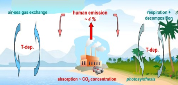
This new paper finds that CO2 concentration in the atmosphere has risen by 110 ppm since 1750, but of this the human contribution is just 17 ppm. With the concentration now at 400 ppm, the human contribution is just 4.3%. The results indicate that almost all of the observed change of CO2 during the Industrial Era comes, not from anthropogenic emissions, but from changes of natural emission.

The general assumption by IPCC and the global warming fraternity that natural carbon dioxide absorption and emissions are miraculously in balance and, therefore that man-made emissions are solely responsible for the increase in carbon dioxide concentration is deeply flawed (if not plain stupid).

Clearly this paper is not at all to the liking of the religious zealots of the “global warming brigade” and is causing much heartburn among the faithful.

Hermann Harde, Scrutinizing the carbon cycle and CO2 residence time in the atmosphereGlobal and Planetary Change, http://dx.doi.org/10.1016/j.gloplacha.2017.02.009

Highlights

•An alternative carbon cycle is presented in agreement with the carbon 14 decay.
•The CO2 uptake rate scales proportional to the CO2 concentration.
•Temperature dependent natural emission and absorption rates are considered.
•The average residence time of CO2 in the atmosphere is found to be 4 years.
•Paleoclimatic CO2 variations and the actual CO2 growth rate are well-reproduced.
•The anthropogenic fraction of CO2 in the atmosphere is only 4.3%.
•Human emissions only contribute 15% to the CO2 increase over the Industrial Era.

AbstractClimate scientists presume that the carbon cycle has come out of balance due to the increasing anthropogenic emissions from fossil fuel combustion and land use change. This is made responsible for the rapidly increasing atmospheric CO2 concentrations over recent years, and it is estimated that the removal of the additional emissions from the atmosphere will take a few hundred thousand years. Since this goes along with an increasing greenhouse effect and a further global warming, a better understanding of the carbon cycle is of great importance for all future climate change predictions. We have critically scrutinized this cycle and present an alternative concept, for which the uptake of CO2 by natural sinks scales proportional with the CO2 concentration. In addition, we consider temperature dependent natural emission and absorption rates, by which the paleoclimatic CO2 variations and the actual CO2 growth rate can well be explained. The anthropogenic contribution to the actual CO2 concentration is found to be 4.3%, its fraction to the CO2 increase over the Industrial Era is 15% and the average residence time 4 years.

Conclusions.

Climate scientists assume that a disturbed carbon cycle, which has come out of balance by the increasing anthropogenic emissions from fossil fuel combustion and land use change, is responsible for the rapidly increasing atmospheric CO2 concentrations over recent years. While over the whole Holocene up to the entrance of the Industrial Era (1750) natural emissions by heterotrophic processes and fire were supposed to be in equilibrium with the uptake by photosynthesis and the net oceanatmosphere gas exchange, with the onset of the Industrial Era the IPCC estimates that about 15 – 40 % of the additional emissions cannot further be absorbed by the natural sinks and are accumulating in the atmosphere.

The IPCC further argues that CO2 emitted until 2100 will remain in the atmosphere longer than 1000 years, and in the same context it is even mentioned that the removal of human-emitted CO2 from the atmosphere by natural processes will take a few hundred thousand years (high confidence) (see AR5-Chap.6-Executive-Summary).

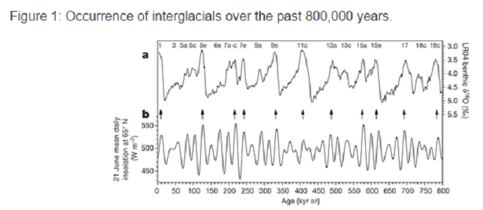
Since the rising CO2 concentrations go along with an increasing greenhouse effect and, thus, a further global warming, a better understanding of the carbon cycle is a necessary prerequisite for all future climate change predictions. In their accounting schemes and models of the carbon cycle the IPCC uses many new and detailed data which are primarily focussing on fossil fuel emission, cement fabrication or net land use change (see AR5-WG1-Chap.6.3.2), but it largely neglects any changes of the natural emissions, which contribute to more than 95 % to the total emissions and by far cannot be assumed to be constant over longer periods (see, e.g.: variations over the last 800,000 years (Jouzel et al., 2007); the last glacial termination (Monnin et al., 2001); or the younger Holocene (Monnin et al., 2004; Wagner et al., 2004)).

Since our own estimates of the average CO2 residence time in the atmosphere differ by several orders of magnitude from the announced IPCC values, and on the other hand actual investigations of Humlum et al. (2013) or Salby (2013, 2016) show a strong relation between the natural CO2 emission rate and the surface temperature, this was motivation enough to scrutinize the IPCC accounting scheme in more detail and to contrast this to our own calculations.

Different to the IPCC we start with a rate equation for the emission and absorption processes, where the uptake is not assumed to be saturated but scales proportional with the actual CO2 concentration in the atmosphere (see also Essenhigh, 2009; Salby, 2016). This is justified by the observation of an exponential decay of 14C. A fractional saturation, as assumed by the IPCC, can directly be expressed by a larger residence time of CO2 in the atmosphere and makes a distinction between a turnover time and adjustment time needless. Based on this approach and as solution of the rate equation we derive a concentration at steady state, which is only determined by the product of the total emission rate and the residence time. Under present conditions the natural emissions contribute 373 ppm and anthropogenic emissions 17 ppm to the total concentration of 390 ppm (2012). For the average residence time we only find 4 years.

The stronger increase of the concentration over the Industrial Era up to present times can be explained by introducing a temperature dependent natural emission rate as well as a temperature affected residence time. With this approach not only the exponential increase with the onset of the Industrial Era but also the concentrations at glacial and cooler interglacial times can well be reproduced in full agreement with all observations. So, different to the IPCC’s interpretation the steep increase of the concentration since 1850 finds its natural explanation in the self accelerating processes on the one hand by stronger degassing of the oceans as well as a faster plant growth and decomposition, on the other hand by an increasing residence time at reduced solubility of CO2 in oceans.

Together this results in a dominating temperature controlled natural gain, which contributes about 85 % to the 110 ppm CO2 increase over the Industrial Era, whereas the actual anthropogenic emissions of 4.3 % only donate 15 %. These results indicate that almost all of the observed change of CO2 during the Industrial Era followed, not from anthropogenic emission, but from changes of natural emission.

The results are consistent with the observed lag of CO2 changes behind temperature changes (Humlum et al., 2013; Salby, 2013), a signature of cause and effect. Our analysis of the carbon cycle, which exclusively uses data for the CO2 concentrations and fluxes as published in AR5, shows that also a completely different interpretation of these data is possible, this in complete conformity with all observations and natural causalities. 

I expect there will be a concerted effort by the faithful to try and debunk this (and it has already started).

But I am inclined to give credence to this work – and not merely because it is in general agreement with my own conclusions about the Carbon cycle. Back in 2013 I posted

Even though the combustion of fossil fuels only contributes less than 4% of total carbon dioxide production (about 26Gt/year of 800+GT/year), it is usually assumed that the sinks available balance the natural sources and that the carbon dioxide concentration – without the effects of man – would be largely in equilibrium.  (Why carbon dioxide concentration should not vary naturally escapes me!). It seems rather illogical to me to claim that sinks can somehow distinguish the source of carbon dioxide in the atmosphere and preferentially choose to absorb natural emissions and reject anthropogenic emissions! Also, there is no sink where the absorption rate would not increase with concentration.

Carbon dioxide emission sources (GT CO2/year)

  • Transpiration 440
  • Release from oceans 330
  • Fossil fuel combustion 26
  • Changing land use 6
  • Volcanoes and weathering 1

Carbon dioxide is accumulating in the atmosphere by about 15 GT CO2/ year. The accuracy of the amounts of carbon dioxide emitted by transpiration and by the oceans is no better than about 2 – 3% and that error band (+/- 20GT/year)  is itself almost as large as the total amount of emissions from fossil fuels.


Risk of rapid North Atlantic cooling in 21st century greater than previously estimated

February 25, 2017

This paper in Nature would not have have had any chance of being published a few years ago. But times are changing.

CNRS: “The possibility of major climate change in the Atlantic region has long been recognized and has even been the subject of a Hollywood movie: The Day After Tomorrow. To evaluate the risk of such climate change, researchers from the Environnements et Paléoenvironnements Océaniques et Continentaux laboratory (CNRS/University of Bordeaux) and the University of Southampton developed a new algorithm to analyze the 40 climate models considered by the latest report from the Intergovernmental Panel on Climate Change (IPCC). Their findings raise the probability of rapid North Atlantic cooling during this century to nearly 50%. Nature Communications publishes their work on February 15, 2017”.

My own view is that man-made global warming is insignificant and virtually impossible to measure. The apparent climate turbulence we may currently be experiencing is probably the exhibition of instabilities as climate shifts from an interglacial paradigm to the, more normal, glacial conditions. The transition will probably be “rapid” in geologic terms which probably means a thousand years or so. Major volcanic eruptions (VEI>6) are overdue. This interglacial has lasted some 13,000 years and is also, relatively, long. I think it feasible that 2 or 3 major volcanic eruptions in relatively quick succession could provide the conditions to trigger a full transition. Once glacial conditions are established they will last for about 100,000 years. And we will then be very thankful for all the fossil or nuclear energy we can have available to us.

Giovanni Sgubin, Didier Swingedouw, Sybren Drijfhout, Yannick Mary, Amine Bennabi. Abrupt cooling over the North Atlantic in modern climate models. Nature Communications, 2017; 8 DOI: 10.1038/ncomms14375

Abstract: Observations over the 20th century evidence no long-term warming in the subpolar North Atlantic (SPG). This region even experienced a rapid cooling around 1970, raising a debate over its potential reoccurrence. Here we assess the risk of future abrupt SPG cooling in 40 climate models from the fifth Coupled Model Intercomparison Project (CMIP5). Contrary to the long-term SPG warming trend evidenced by most of the models, 17.5% of the models (7/40) project a rapid SPG cooling, consistent with a collapse of the local deep-ocean convection. Uncertainty in projections is associated with the models’ varying capability in simulating the present-day SPG stratification, whose realistic reproduction appears a necessary condition for the onset of a convection collapse. This event occurs in 45.5% of the 11 models best able to simulate the observed SPG stratification. Thus, due to systematic model biases, the CMIP5 ensemble as a whole underestimates the chance of future abrupt SPG cooling, entailing crucial implications for observation and adaptation policy.

Even The Guardian (a high priest of the man-made global warming religious fantasy) is compelled to report!!

guardian-global-cooling


CNRS Press Release:

Current climate models all foresee a slowing of the meridional overturning circulation (MOC)2—the phenomenon behind the familiar Gulf Stream, which carries warmth from Florida to European shores—that could lead to a dramatic, unprecedented disruption of the climate system. In 2013, drawing on 40 climate change projections, the IPCC judged that this slowdown would occur gradually over a long period of time. The panel’s findings suggested that fast cooling of the North Atlantic during this century was unlikely.

Oceanographers from the EU EMBRACE project team reexamined the 40 projections by focusing on a critical spot in the northwest North Atlantic: the Labrador Sea. The Labrador Sea is host to a convection system ultimately feeding into the ocean-wide MOC. The temperatures of its surface waters plummet in the winter, increasing their density and causing them to sink. This displaces deep waters, which bring their heat with them as they rise to the surface, preventing the formation of ice caps. To investigate this phenomenon in greater detail, the researchers developed an algorithm able to detect quick sea surface temperature variations. Their number crunching revealed that 7 of the 40 climate models they were studying predicted total shutdown of convection, leading to abrupt cooling of the Labrador Sea: by 2–3 °C over less than 10 years. This in turn would drastically lower North Atlantic coastal temperatures.

But is such rapid cooling a real possibility? (After all, only a handful of the models supported this projection.) To answer this question, the researchers honed in on the critical parameter triggering winter convection: ocean stratification. Indeed, 11 of the 40 models incorporated vertical variation in the density of oceanic water masses. And of these 11 models, which we may furthermore consider to be the most reliable, 5 (i.e., 45% of the models) predicted a rapid drop in North Atlantic temperatures.  


Conundrums

February 24, 2017

Not that these keep me awake at night, but they do irritate.

conundrums-1


A model to explain the end of an ice age (but not yet to predict when one may start)

February 23, 2017

That the onset of glacial (cold) and interglacial (warm) periods on earth are a consequence of the Milankovitch cycles is almost certain. Researchers have now developed a model which seems to be able to explain why and when glacial periods end to give interglacial conditions. Exactly what cause glacial conditions to be triggered remains to be discovered.

P. C. Tzedakis, M. Crucifix, T. Mitsui, E. W. Wolff. A simple rule to determine which insolation cycles lead to interglacials. Nature, 2017; 542 (7642): 427 DOI: 10.1038/nature21364

AbstractThe pacing of glacial–interglacial cycles during the Quaternary period (the past 2.6 million years) is attributed to astronomically driven changes in high-latitude insolation. However, it has not been clear how astronomical forcing translates into the observed sequence of interglacials. Here we show that before one million years ago interglacials occurred when the energy related to summer insolation exceeded a simple threshold, about every 41,000 years. Over the past one million years, fewer of these insolation peaks resulted in deglaciation (that is, more insolation peaks were ‘skipped’), implying that the energy threshold for deglaciation had risen, which led to longer glacials. However, as a glacial lengthens, the energy needed for deglaciation decreases. A statistical model that combines these observations correctly predicts every complete deglaciation of the past million years and shows that the sequence of interglacials that has occurred is one of a small set of possibilities. The model accounts for the dominance of obliquity-paced glacial–interglacial cycles early in the Quaternary and for the change in their frequency about one million years ago. We propose that the appearance of larger ice sheets over the past million years was a consequence of an increase in the deglaciation threshold and in the number of skipped insolation peaks.

Onset of Interglacials Tzedakis et al

Onset of Interglacials Tzedakis et al

Science Daily reports:

…. In a new study published today in Nature, researchers from UCL (University College London), University of Cambridge and University of Louvain have combined existing ideas to solve the problem of which solar energy peaks in the last 2.6 million years led to the melting of the ice sheets and the start of a warm period.

During this interval, Earth’s climate has alternated between cold (glacial) and warm (interglacial) periods. In the cold times, ice sheets advanced over large parts of North America and northern Europe. In the warm periods like today, the ice sheets retreated completely.

It has long been realised that these cycles were paced by astronomical changes in the Earth’s orbit around the Sun and in the tilt of its axis, which change the amount of solar energy available to melt ice at high northern latitudes in summer.

However, of the 110 incoming solar energy peaks (about every 21,000 years) only 50 led to complete melting of the ice sheets. Finding a way to translate the astronomical changes into the sequence of interglacials has previously proved elusive. 

Professor Chronis Tzedakis (UCL Geography) said: “The basic idea is that there is a threshold for the amount of energy reaching high northern latitudes in summer. Above that threshold, the ice retreats completely and we enter an interglacial.”

From 2.6 to 1 million years ago, the threshold was reached roughly every 41,000 years, and this predicts almost perfectly when interglacials started and the ice sheets disappeared. Professor Eric Wolff (University of Cambridge) said: “Simply put, every second solar energy peak occurs when the Earth’s axis is more inclined, boosting the total energy at high latitudes above the threshold.”

Somewhere around a million years ago, the threshold rose, so that the ice sheets kept growing for longer than 41,000 years. However, as a glacial period lengthens, ice sheets become larger, but also more unstable.

The researchers combined these observations into a simple model, using only solar energy and waiting time since the previous interglacial, that was able to predict all the interglacial onsets of the last million years, occurring roughly every 100,000 years.

Dr Takahito Mitsui (University of Louvain) said: “The next step is to understand why the energy threshold rose around a million years ago — one idea is that this was due to a decline in the concentration of CO2, and this needs to be tested.”

The results explain why we have been in a warm period for the last 11,000 years: despite the weak increase in solar energy, ice sheets retreated completely during our current interglacial because of the very long waiting time since the previous interglacial and the accumulated instability of ice sheets. …..

Milankovitch Cycles (Wikipedia)

What would cause the current interglacial to end remains to be discovered. It’s only my speculation of course but I suspect that a trigger event is probably needed. Possibly 2 or 3 major (VEI >6) volcanic eruptions over a short period, with large amounts of dust, which in turn led to a a few “years without summers”, could provide such a trigger for an unstoppable process. However the onset of full glacial conditions would still take a few thousand years. The availability of high energy densities would probably make it (relatively) easy for humans to continue to thrive and prosper (as they have done through other glacial periods with much lower energy availability).