Posts Tagged ‘climate models’

Judith Curry’s guide to climate models

November 13, 2016

Judith Curry’s guide to climate models.

Well worth reading.

Though written for lawyers, it might even be tough for many lawyers. However politicians should get their “science” aides to read, digest and summarise it for them (it would be far too ambitious to expect the politicians to be able to read so much, understand it or to digest so much in one go).

For me, the real issue with GCM’s is not that the modelling is done but that they are used for policy making. Assumed sensitivities are effectively used to fit the results for the immediate past. The forced fit is then taken as proof that the assumptions are true and are then projected into the future. The claimed objective of the resultant policies can neither be monitored nor measured.


Climate models for lawyers

by Judith Curry

I have been asked to write an Expert Report on climate models.

No, I can’t tell you the context for this request (at this time, anyways).  But the audience is lawyers.

Here are the specific questions I have been asked to respond to:

  1. What is a Global Climate Model (GCM)?
  2. What is the reliability of climate models?
  3. What are the failings of climate models?
  4. Are GCM’s are a reliable tool for predicting climate change?

I’ve appended my draft Report below. I tried to avoid giving a ‘science lesson’, and focus on what climate models can and can’t do, focusing on policy relevant applications of climate models.  I’ve tried write an essay that would be approved by most climate modelers; at the same time, it has to be understandable by lawyers. I would greatly appreciate your feedback on:

  • whether you think lawyers will understand this
  • whether the arguments I’ve made are the appropriate ones
  • whether I’m missing anything
  • anything that could be left out (its a bit long).

——–

What is a Global Climate Model (GCM)?

Global climate models (GCMs) simulate the Earth’s climate system, with modules that simulate the atmosphere, ocean, land surface, sea ice and glaciers.  The atmospheric module simulates evolution of the winds, temperature, humidity and atmospheric pressure using complex mathematical equations that can only be solved using computers. These equations are based on fundamental physical principles, such as Newton’s Laws of Motion and the First Law of Thermodynamics.

GCMs also include mathematical equations describing the three-dimensional oceanic circulation, how it transports heat, and how the ocean exchanges heat and moisture with the atmosphere. Climate models include a land surface model that describes how vegetation, soil, and snow or ice cover exchange energy and moisture with the atmosphere. GCMs also include models of sea ice and glacier ice.

To solve these equations on a computer, GCMs divide the atmosphere, oceans, and land into a 3-dimensional grid system (see Figure 1). The equations and are then calculated for each cell in the grid repeatedly for successive time steps that march forward in time throughout the simulation period.

slide1

Figure 1. Schematic of a global climate model.

The number of cells in the grid system determines the model ‘resolution.’ Common resolutions for a GCM include a horizontal resolution of about 100-200 km, a vertical resolution of about 1 km, and a time stepping resolution that is typically about 30 minutes. While GCMs represent processes more realistically at higher resolution, the computing time required to do the calculations increases substantially at higher resolutions. The coarseness of the model resolution is driven by the available computer resources, and tradeoffs between model resolution, model complexity and the length and number of simulations to be conducted.

Because of the relatively coarse spatial and temporal resolutions of the models, there are many important processes that occur on scales that are smaller than the model resolution (such as clouds and rainfall; see inset in Figure 1). These subgrid-scale processes are represented using ‘parameterizations.’ Parameterizations of subgrid-scale processes are simple formulas based on observations or derivations from more detailed process models. These parameterizations are ‘calibrated’ or ‘tuned’ so that the climate models perform adequately when compared with historical observations.

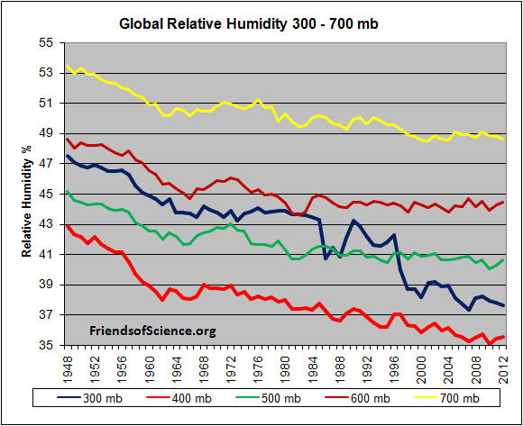
The actual equations used in the GCM computer codes are only approximations of the physical processes that occur in the climate system. While some of these approximations are highly accurate, others are unavoidably crude. This is because the real processes they represent are either poorly understood or too complex to include in the model given the constraints of the computer system. Of the processes that are most important for climate change, parameterizations related to clouds and precipitation remain the most challenging, and are the greatest source of disagreement among different GCMs.

GCMs are used for the following purposes:

  • Simulation of present and past climate states to understand planetary energetics and other complex interactions
  • Numerical experiments to understand how the climate system works. Sensitivity experiments are used to turn off, constrain or enhance certain physical processes or external forcings (e.g. CO2, volcanoes, solar output) to see how the system responds.
  • Understanding the causes of past climate variability and change (e.g. how much of the change can be attributed to human causes such as CO2, versus natural causes such as solar variations, volcanic eruptions, and slow circulations in the ocean).
  • Simulation of future climate states, from decades to centuries, e.g. simulations of future climate states under different emissions scenarios.
  • Prediction and attribution of the statistics extreme weather events (e.g. heat waves, droughts, hurricanes)
  • Projections of future regional climate variations to support decision making related adaptation to climate change
  • Guidance for emissions reduction policies
  • Projections of future risks of black swan events (e.g. climate surprises)

The specific objectives of a GCM vary with purpose of the simulation. Generally, when simulating the past climate using a GCM, the objective is to correctly simulate the spatial variation of climate conditions in some average sense.  When predicting future climate, the aim is not to simulate conditions in the climate system on any particular day, but to simulate conditions over a longer period—typically decades or more—in such a way that the statistics of the simulated climate will match the statistics of the actual future climate.

There are more than 20 climate modeling groups internationally, that contribute climate model simulations to the IPCC Assessment Reports. Further, many of the individual climate modeling groups contribute simulations from multiple different models. Why are there so many different climate models? Is it possible to pick a ‘best’ climate model?

There are literally thousands of different choices made in the construction of a climate model (e.g. resolution, complexity of the submodels, parameterizations). Each different set of choices produces a different model having different sensitivities. Further, different modeling groups have different focal interests, e.g. long paleoclimate simulations, details of ocean circulations, nuances of the interactions between aerosol particles and clouds, the carbon cycle. These different interests focus computational resources on a particular aspect of simulating the climate system, at the expense of others.

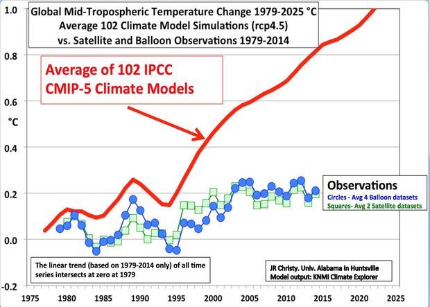
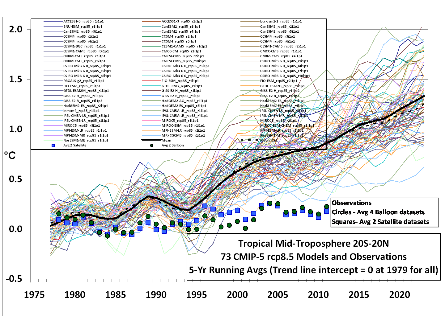
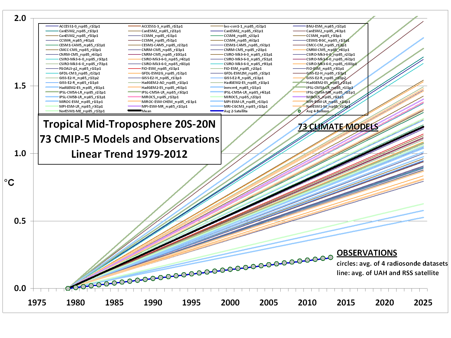
Is it possible to select a ‘best’ model? Well, several models generally show a poorer performance overall when compared with observations. However, the best model depends on how you define ‘best’, and no single model is the best at everything. The more germane issue is to assess model’s ‘fitness for purpose’, which is addressed in Sections 2-4.

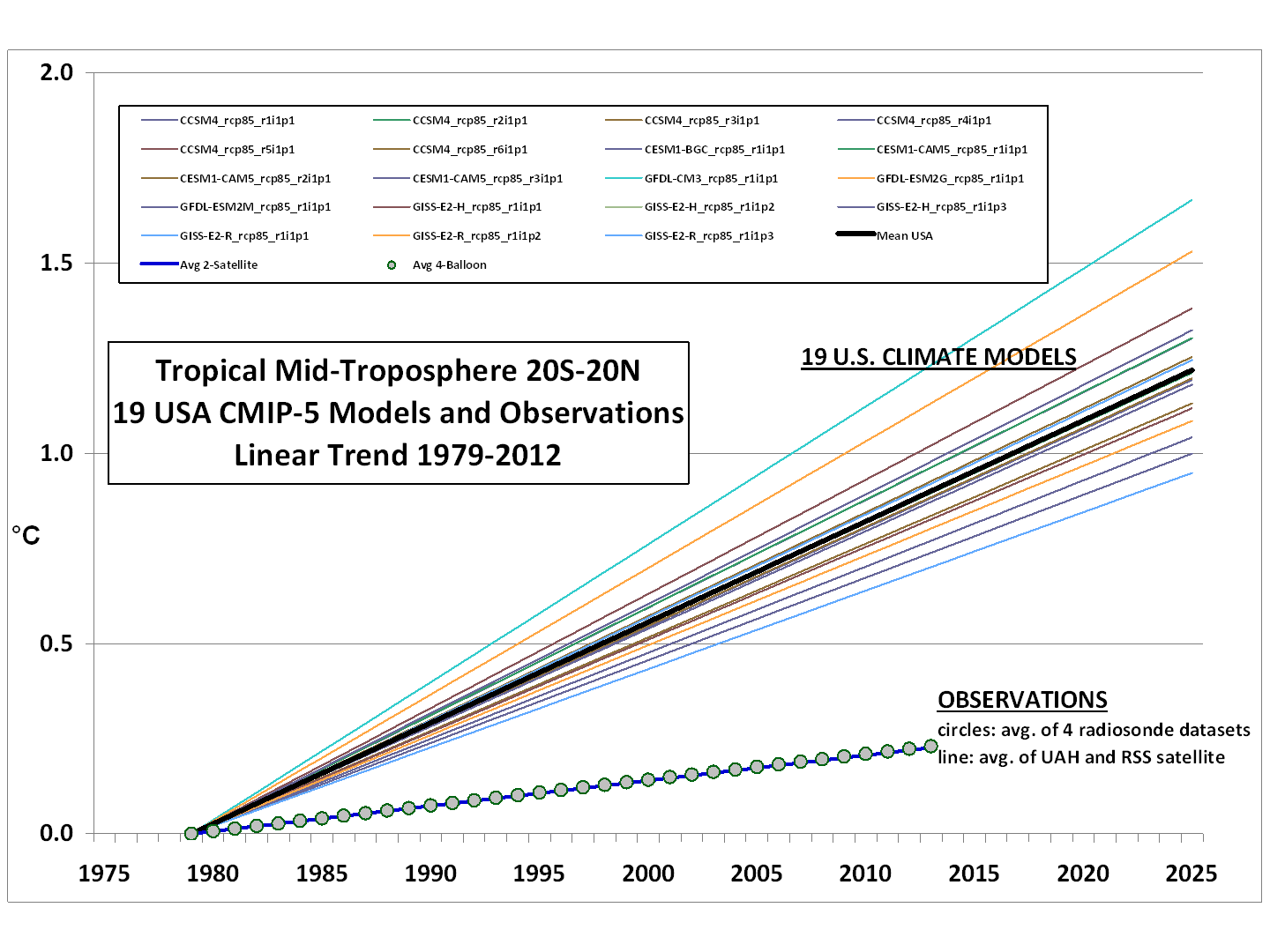
The reliability of climate models ……


Read the whole post

at https://judithcurry.com/2016/11/12/climate-models-for-lawyers/


Climate models would fit data better if they drastically reduced carbon dioxide “forcings”

August 9, 2015

It is almost the first lesson I was taught when I started doing “research”. Research 101. If the data does not fit the model, you change the model – not the data. The fundamental problem with climate models is that they are not falsifiable. And as long as “climate science” can not, or will not, put forward falsifiable hypotheses, it is not Science. The models all start with assumptions which are approved by the high-priests of the religion. The results are then “forced” to fit with past data and are then used to assert that the initial assumptions are correct. When they are then used for making forecasts they invariably fail. They then try to “adjust” the data (cooling the past) rather than change their religiously-held assumptions.

Five year running mean temperatures predicted by UN IPCC models and observations by weather balloons and satellites. University of Alabama’s John Christy presentation to the House Committee on Natural Resources on May 15, 2015.

Five year running mean temperatures predicted by UN IPCC models and observations by weather balloons and satellites. University of Alabama’s John Christy presentation to the House Committee on Natural Resources on May 15, 2015.

Just the effect of carbon dioxide concentration on incoming and outgoing radiation is small, easy to include and not really an issue. The problem arises because of the assumptions made of the feedback loops and the subsequent “forcing” attributed to carbon dioxide concentration. It is politically incorrect and therefore no climate model is ever allowed to ignore carbon dioxide “forcings”. Even though the “forcings” are largely conjecture. The feedback loops due to changes in carbon dioxide concentration acting through consequent changes in water vapour concentration and cloud cover are not only not known – it is not even known if they are net positive or net negative on temperature. The unknown “forcings” are called “climate sensitivity”, just to make it sound better, but these “climate sensitivities” are little better than fudge factors used by each model. (Even more fudge factors are applied to assert how man-made carbon dioxide emissions affect the carbon dioxide concentration even though the long-term data show that carbon dioxide concentration lags temperature). What I note is that the error between the models and real data is of the same magnitude as ascribed to the effects – with “forcing” – of carbon dioxide concentration in the atmosphere. There is no evidence that the assumed “forcings” are valid. The obvious correction to be made in the model assumptions is that the “climate sensitivity” assumed for carbon dioxide concentration is too high and that any “forcing” effects must be scaled down. But that, of course, is politically incorrect. You cannot get funding for developing a model which does not pay homage to the orthodoxy.

A simple sanity check shows that every single climate model used by the UN’s IPCC would fit real data better if it used a much lower sensitivity to carbon dioxide concentration by using a lower level of assumed forcing.

If the globe is warming how come relative humidity is decreasing?

August 22, 2014

Increasing temperature leads to a greater capacity for air to hold moisture (the specific humidity). The actual amount of moisture held in a sample of air as a proportion of the capacity of that air to hold moisture is termed the relative humidity and is usually given as a percentage.

Specific humidity (g/kg) versus temperature for air  earthobservatory.nasa.gov

All climate computer models usually assume a constant relative humidity.

NasaIn climate modeling, scientists have assumed that the relative humidity of the atmosphere will stay the same regardless of how the climate changes. In other words, they assume that even though air will be able to hold more moisture as the temperature goes up, proportionally more water vapor will be evaporated from the ocean surface and carried through the atmosphere so that the percentage of water in the air remains constant. Climate models that assume that future relative humidity will remain constant predict greater increases in the Earth’s temperature in response to increased carbon dioxide than models that allow relative humidity to change. The constant-relative-humidity assumption places extra water in the equation, which increases the heating.

Relative humidity has decreased steadily for over 60 years. All computer models which assume constant relative humidity will overestimate the feedback and the degree of warming.

Forbes carries an article about the mismatch between computer models and actual observations.

ForbesWater vapor is a much more potent greenhouse gas than carbon dioxide, so substantial increases in atmospheric water vapor can certainly cause significant warming. United Nations computer models are programmed to assume that absolute humidity (the total amount of water vapor in the atmosphere) will rise so much that even relative humidity (the percent of water vapor in the atmosphere) will at least keep pace and perhaps even increase. Warmer air is able to hold more water than cooler air, so absolute water vapor would have to increase quite substantially for relative humidity to remain constant or increase in a warming world.

Scientists, however, have been measuring relative humidity for many decades. Rather than keeping pace with modestly warming temperatures, relative humidity is declining. This decline has been ongoing, without interruption, for more than 60 years. After more than six decades of consistent data, we can say with strong confidence that absolute humidity is not rising rapidly enough for relative humidity to keep pace with warming temperatures.

Global Relative Humidity 300 -700mb

Global Relative Humidity 300 – 700mb  (300mb corresponds to about 9,000 m altitude)

The failure of relative humidity to hold constant or rise during recent decades is a lethal dagger in the heart of alarmist global warming claims. According to the UN computer models, rapidly rising absolute humidity will cause substantially more global warming than the modest warming directly caused by rising carbon dioxide levels. Given the potency of water vapor, even a small overstatement of atmospheric humidity levels in UN computer models will cause a very significant overstatement of future warming. And the data show UN computer models assume too much atmospheric humidity.

The effects of this overstatement are apparent in real-world temperature data this century. Precise atmospheric temperature measurements compiled by NASA and NOAA satellite instruments show there has been no global warming since late in the 20th century


Climate modelling: Study shows that without access to water fish will die!

August 21, 2014

I am sure all the forecasts based on climate models applied to hydrological models and extrapolated to 2050 are all quite clever. But it is no evidence of anything.

I am not sure why their conclusions are confined to Arizona. I suspect it may be a profound and universal truth that: Without water fish will die!!

My reading of this study (which I put under Trivia):

If the climate develops as we have modelled,

and if the surface water flows are reduced,

and if the connectivity of the water streams is reduced as we have modelled,

then some fish will lose access to water,

and some of those fish will die.

K. L. Jaeger, J. D. Olden, N. A. Pelland. Climate change poised to threaten hydrologic connectivity and endemic fishes in dryland streams. Proceedings of the National Academy of Sciences, 2014; DOI: 10.1073/pnas.1320890111

Significance (In other words an abstract of the abstract)

We provide the first demonstration to our knowledge that projected changes in regional climate regimes will have significant consequences for patterns of intermittence and hydrologic connectivity in dryland streams of the American Southwest. By simulating fine-resolution streamflow responses to forecasted climate change, we simultaneously evaluate alterations in local flow continuity over time and network flow connectivity over space and relate how these changes may challenge the persistence of a globally endemic fish fauna. Given that human population growth in arid regions will only further increase surface and groundwater extraction during droughts, we expect even greater likelihood of flow intermittence and loss of habitat connectivity in the future.

(my bold)

The University of Ohio goes to town with its Press Release : Climate Change will threaten fish…

Fish species native to a major Arizona watershed may lose access to important segments of their habitat by 2050 as surface water flow is reduced by the effects of climate warming, new research suggests. ….. 

“If water is flowing throughout the network, fish are able to access all parts of it and make use of whatever resources are there. But when systems dry down, temporary fragmented systems develop that force fish into smaller, sometimes isolated channel reaches or pools until dry channels wet up again.”…….


The IPCC 95% trick: Increase the uncertainty to increase the certainty

October 17, 2013

Increasing the uncertainty in a statement to make the statement more certain to be applicable is an old trick of rhetoric. Every politician knows how to use that in a speech. It is a schoolboy’s natural defense when being hauled up for some wrongdoing. It is especially useful when caught in a lie. It is the technique beloved of defense lawyers in TV dramas. Salesmen are experts at this. It is standard practice in scientific publications when experimental data does not fit the original hypothesis.

Modify the original statement (the lie) to be less certain in the lie, so as to be more certain that the statement could be true. Widen the original hypothesis to encompass the actual data. Increase the spread of the deviating model results to be able to include the real data within the error envelope.

  • “I didn’t say he did it. I said somebody like him could have done it”
  • “Did you start the fight?” >>> “He hit me back first”.
  • “The data do not match your hypothesis” >>> “The data are not inconsistent with the improved hypothesis”
  • “Your market share has reduced” >>> “On the contrary, our market share of those we sell to has increased!” (Note -this is an old one used by salesmen to con “green” managers with reports of a 100% market share!!)

And it is a trick that is not foreign to the IPCC  – “we have a 95% certainty that the less reliable (= improved) models are correct”. Or in the case of the Cook consensus “97% of everybody believes that climate does change”.

A more rigorous treatment of the IPCC trick is carried out by Climate Audit and Roy Spencer among others but this is my simplified explanation for schoolboys and Modern Environ-mentalists.

The IPCC Trick

The IPCC Trick

The real comparison between climate models and global temperatures is below:

Climate Models and Reality

Climate Models and Reality

With the error in climate models increased to infinity, the IPCC could even reach 100% certainty. As it is the IPCC is 95% certain that it is warming – or not!

Integrated Assessment Climate models tell us “very little”

August 24, 2013

Mathematical models are used – and used successfully – everyday in Engineering, Science, Medicine and Business. Their usefulness is determined – and some are extremely useful – by knowing their limitations and acknowledging that they only represent an approximation of real complex systems.  Actual measurements always override the model results and whenever reality does not agree with model predictions it is usually mandatory to adjust the model. Where the adjustments can only be made by using “fudge factors” it is usually necessary to revisit the simplifying assumptions used to formulate the model in the first place.

But this is not how Climate Modelling Works. Reality or actual measurements are not allowed to disturb the model or its results for the far future. Fudge factors galore are introduced to patch over the differences when they appear. The adjustments to the model are just sufficient to cover the observed difference to reality but such that the long-term “result” is maintained.

The assumption that carbon dioxide has a significant role to play in global warming is itself hypothetical. Climate models start with that as an assumption. They don’t address whether there is a link between the two. Some level of warming is assumed to be the consequence of a doubling the carbon dioxide concentration in the atmosphere. For the last 17 years global temperature has stood still while carbon dioxide concentration has increased dramatically. There is actually more evidence to hypothesise that there is no link (or a very weak link) between carbon dioxide and global warming than that there is. Nevertheless all climate models start with the built-in assumption that the link exists. And then use the results of the model as proof that the link exists! They are not just cyclical arguments – they are incestuous – or do I mean cannibalistic.

It is bad enough that economic models, developed to count the cost of carbon dioxide are first based on some hypothetical magnitude of the link between carbon dioxide emission and global warming as their starting point. But it gets worse. These “integrated assessment” models then themselves are strewn with new assumptions and further cyclical logic as to how the costs ensue.

A new paper by Prof. Robert Pindyck for the National Bureau of Economic Research takes a less than admiring look at the Integrated Assessment Climate models and their uselessness.

Robert S. PindyckClimate Change Policy: What Do the Models Tell Us?, NBER Working Paper No. 19244
Issued in July 2013

(A pdf of the full paper is here: Climate-Change-Policy-What-Do-the-Models-Tell-Us)

Abstract: Very little. A plethora of integrated assessment models (IAMs) have been constructed and used to estimate the social cost of carbon (SCC) and evaluate alternative abatement policies. These models have crucial flaws that make them close to useless as tools for policy analysis: certain inputs (e.g. the discount rate) are arbitrary, but have huge effects on the SCC estimates the models produce; the models’ descriptions of the impact of climate change are completely ad hoc, with no theoretical or empirical foundation; and the models can tell us nothing about the most important driver of the SCC, the possibility of a catastrophic climate outcome. IAM-based analyses of climate policy create a perception of knowledge and precision, but that perception is illusory and misleading.

Even though his assumptions about “climate sensitivity” are somewhat optimistic, he is more concerned with the assumptions made to try and develop the “damage” function to enable the cost to be estimated:

When assessing climate sensitivity, we at least have scientific results to rely on, and can argue coherently about the probability distribution that is most consistent with those results. When it comes to the damage function, however, we know almost nothing, so developers of IAMs [Integrated Assessment Models] can do little more than make up functional forms and corresponding parameter values. And that is pretty much what they have done. …..  

But remember that neither of these loss functions is based on any economic (or other) theory. Nor are the loss functions that appear in other IAMs. They are just arbitrary functions, made up to describe how GDP goes down when T goes up.

…. Theory can’t help us, Nor is data available that could be used to estimate or even roughly calibrate the parameters. As a result, the choice of values for these parameters is essentially guesswork. The usual approach is to select values such that L(T ) for T in the range of 2◦C to 4◦C is consistent with common wisdom regarding the damages that are likely to occur for small to moderate increases in temperature.

…… For example, Nordhaus (2008) points out (page 51) that the 2007 IPCC report states that “global mean losses could be 1–5% GDP for 4◦C of warming.” But where did the IPCC get those numbers? From its own survey of several IAMs. Yes, it’s a bit circular. 

The bottom line here is that the damage functions used in most IAMs are completely made up, with no theoretical or empirical foundation. That might not matter much if we are looking at temperature increases of 2 or 3◦C, because there is a rough consensus (perhaps completely wrong) that damages will be small at those levels of warming. The problem is that these damage functions tell us nothing about what to expect if temperature increases are larger, e.g., 5◦C or more.19 Putting T = 5 or T = 7 into eqn. (3) or (4) is a completely meaningless exercise. And yet that is exactly what is being done when IAMs are used to analyze climate policy.

And he concludes:

I have argued that IAMs are of little or no value for evaluating alternative climate change policies and estimating the SCC. On the contrary, an IAM-based analysis suggests a level of knowledge and precision that is nonexistent, and allows the modeler to obtain almost any desired result because key inputs can be chosen arbitrarily. 

As I have explained, the physical mechanisms that determine climate sensitivity involve crucial feedback loops, and the parameter values that determine the strength of those feedback loops are largely unknown. When it comes to the impact of climate change, we know even less. IAM damage functions are completely made up, with no theoretical or empirical foundation. They simply reflect common beliefs (which might be wrong) regarding the impact of 2◦C or 3◦C of warming, and can tell us nothing about what might happen if the temperature increases by 5◦C or more. And yet those damage functions are taken seriously when IAMs are used to analyze climate policy. Finally, IAMs tell us nothing about the likelihood and nature of catastrophic outcomes, but it is just such outcomes that matter most for climate change policy. Probably the best we can do at this point is come up with plausible estimates for probabilities and possible impacts of catastrophic outcomes. Doing otherwise is to delude ourselves.

….

Climate model results depend upon which computer they run on!

June 26, 2013

Robust models indeed.

Washington Post:

New Weather Service supercomputer faces chaos

The National Weather Service is currently in the process of transitioning its primary computer model, the Global Forecast System (GFS), from an old supercomputer to a brand new one.  However, before the switch can be approved, the GFS model on the new computer must generate forecasts indistinguishable from the forecasts on the old one.

One expects that ought not to be a problem, and to the best of my 30+ years of personal experience at the NWS, it has not been.  But now, chaos has unexpectedly become a factor and differences have emerged in forecasts produced by the identical computer model but run on different computers.

This experience closely parallels Ed Lorenz’s experiments in the 1960s, which led serendipitously to development of chaos theory (aka “butterfly effect). What Lorenz found – to his complete surprise – was that forecasts run with identically the same (simplistic) weather forecast model diverged from one another as forecast length increased solely due to even minute differences inadvertently introduced into the starting analyses (“initial conditions”). ..

……

Why averaging climate models is meaningless

June 14, 2013

This comment/ essay by rgbatduke on WUWT is well worth reading and digesting.

“this is a point that is stunningly ignored — there are a lot of different models out there, all supposedly built on top of physics, and yet no two of them give anywhere near the same results!”

A professional taking amateurs to task!

(Note! See also his follow-up comments here and here rgbatduke would seem to be Professor R G Brown of Duke University?)

rgbatduke says:

Saying that we need to wait for a certain interval in order to conclude that “the models are wrong” is dangerous and incorrect for two reasons. First — and this is a point that is stunningly ignored — there are a lot of different models out there, all supposedly built on top of physics, and yet no two of them give anywhere near the same results!

This is reflected in the graphs Monckton publishes above, where the AR5 trend line is the average over all of these models and in spite of the number of contributors the variance of the models is huge. It is also clearly evident if one publishes a “spaghetti graph” of the individual model projections (as Roy Spencer recently did in another thread) — it looks like the frayed end of a rope, not like a coherent spread around some physics supported result.

Note the implicit swindle in this graph — by forming a mean and standard deviation over model projections and then using the mean as a “most likely” projection and the variance as representative of the range of the error, one is treating the differences between the models as if they are uncorrelated random variates causing >deviation around a true mean!.

Say what?

This is such a horrendous abuse of statistics that it is difficult to know how to begin to address it. One simply wishes to bitch-slap whoever it was that assembled the graph and ensure that they never work or publish in the field of science or statistics ever again. One cannot generate an ensemble of independent and identically distributed models that have different code. One might, possibly, generate a single model that generates an ensemble of predictions by using uniform deviates (random numbers) to seed
“noise” (representing uncertainty) in the inputs.

What I’m trying to say is that the variance and mean of the “ensemble” of models is completely meaningless, statistically because the inputs do not possess the most basic properties required for a meaningful interpretation. They are not independent, their differences are not based on a random distribution of errors, there is no reason whatsoever to believe that the errors or differences are unbiased (given that the only way humans can generate unbiased anything is through the use of e.g. dice or other objectively random instruments).

(more…)

The reality of “climate change” for a gardener

June 8, 2013

Reality has this nasty habit of rudely intruding upon climate models – and the pronouncements of august bodies like the IPCC.

Reblogged from Bishop Hill:

A reader kindly points me to the blog of UK seed merchant Thompson and Morgan, where Emma Cooper is wondering what to plant this year:

Over the years in which climate change has been discussed in the media, there have been continual suggestions that it will be of benefit to gardeners – allowing us to grow fruit and vegetable crops that enjoy the continental climate, but fail to thrive in a traditional British summer. As those warm summer days have failed to materialise, and look increasing unlikely, I am eyeing up my new allotment with a view to planting crops that will enjoy our cool climate. ……

But 97% of the world’s “climate scientists” can’t be wrong – can they?

Climate models stretch credulity

June 6, 2013

What is perplexing is the blind faith in the climate models and reluctance to revisit the assumptions on which the clearly fallacious models are based.

UPDATE!!

Dr. Spencer has also provided the “un-linearised” data  and writes:

In response to those who complained in my recent post that linear trends are not a good way to compare the models to observations (even though the modelers have claimed that it’s the long-term behavior of the models we should focus on, not individual years), here are running 5-year averages for the tropical tropospheric temperature, models versus observations (click for full size):
CMIP5-73-models-vs-obs-20N-20S-MT-5-yr-means
In this case, the models and observations have been plotted so that their respective 1979-2012 trend lines all intersect in 1979, which we believe is the most meaningful way to simultaneously plot the models’ results for comparison to the observations.

In my opinion, the day of reckoning has arrived. The modellers and the IPCC have willingly ignored the evidence for low climate sensitivity for many years, despite the fact that some of us have shown that simply confusing cause and effect when examining cloud and temperature variations can totally mislead you on cloud feedbacks (e.g. Spencer & Braswell, 2010). The discrepancy between models and observations is not a new issue…just one that is becoming more glaring over time. ….

….

Reblogged from Dr. Roy Spencer

Courtesy of John Christy, a comparison between 73 CMIP5 models (archived at the KNMI Climate Explorer website) and observations for the tropical bulk tropospheric temperature (aka “MT”) since 1979 (click for large version):
CMIP5-73-models-vs-obs-20N-20S-MT
Rather than a spaghetti plot of the models’ individual years, we just plotted the linear temperature trend from each model and the observations for the period 1979-2012.

Note that the observations (which coincidentally give virtually identical trends) come from two very different observational systems: 4 radiosonde datasets, and 2 satellite datasets (UAH and RSS).

If we restrict the comparison to the 19 models produced by only U.S. research centers, the models are more tightly clustered:
CMIP5-19-USA-models-vs-obs-20N-20S-MT

Now, in what universe do the above results not represent an epic failure for the models?

I continue to suspect that the main source of disagreement is that the models’ positive feedbacks are too strong…and possibly of even the wrong sign.

The lack of a tropical upper tropospheric hotspot in the observations is the main reason for the disconnect in the above plots, and as I have been pointing out this is probably rooted in differences in water vapor feedback. The models exhibit strongly positive water vapor feedback, which ends up causing a strong upper tropospheric warming response (the “hot spot”), while the observation’s lack of a hot spot would be consistent with little water vapor feedback.


%d bloggers like this: